Normal Distribution
Suppose that we have three sets of data, each are generated from a random variable that follow the standard normal
distribution, with 20,1000 and 100,000 samples, respectively. We can partition the horizontal axis which represents the
values of the each data point, into many small intervals. For each small interval, we count the number of data points that
falls inside of it, then calculate the ratio of this number to the total number of data (20, 1000 or 100,000). This ratio will
be an estimate that the value of a random variable X ∼ N(0,1) falls inside the interval (empirical probability). Then we
measure the length of the interval, use it as a base to draw a rectangle with a height so that the area of the rectangle
will be this estimated probability. If we do this for each small intervals of partition and then fit a smooth curve (different
numerical methods or partitions may be used, so the curve may not pass the top of these rectangles) for these bars, then
it will be the graph of an empirical probability density function. See the following example. The data sets are contained
in the file:
Example Figure below plotted (Using Mathematica "Histogram” function with "PDF” option turned on) two versions
of histograms for each of the three data sets mentioned above. The plots for the first row are for the data set that contains
20 values, the plots for the second row are for the data set that contains 1000 values. The last row is for the third data set.
The first column uses relative frequencies (empirical probabilities) as heights for each bar, which is not useful for our
purposes: We want to see the construction of EPDFs, plot both EPDFs and PDFs, then compare them. The curve above
it is the empirical probability density function (EPDF). So obviously for each data sets, the corresponding figures in the
first column do not match.
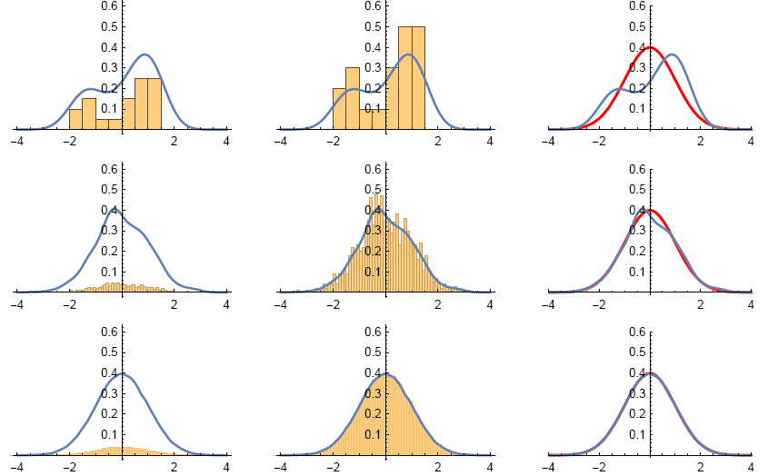
Now look at the plots in the second column of figure 1.5. These figures are histograms that use bar areas to represent
the corresponding empirical probabilities (for each small interval). There are seven bars, each with width 0.5. We now
verify that the areas of each bars is the same as their corresponding empirical probabilities. The intervals that are bases
of the bars are
[−2,−1.5), [−1.5,−1), [−1,−0.5), [−0.5,0), [0,0.5), [0.5,1), [1,1.5).
The following R code will generate histograms similar to the ones shown in the first column of figure 1.5. As for the
data used to get the second picture in the first row, we can just copy and paste. Also the code sorted the data in increasing
order.
According to sorted data, two of the 20 numbers falls inside (−2,−1.5): −1.7813000 and −1.7279600. The relative frequency(empirical probability) is 2/20= 0.1. Thus, we need to make a rectangle with height 0.1/0.5= 0.2 to make its area equal to the relative frequency 0.1.Next, consider the interval (0.5,1). According to sorted data, 5 numbers are inside it. So the relative frequency is 5/20=1/4 . With base 1/2 , we need to make a rectangle with height 1/2 to make its area equal the relative frequency 1/4.
Similarly, we can verify the rest of the rectangles (bars). As we can see, as more and more data points available (from the first row to the last row), empirical probability density function will looks more and more like the theoretical probability density function (see the last column of the figure). The histograms in the second column is a Riemann-sum that should converge to the area under the graph of the probability density function (integral).